Jigsaw Puzzle Problem

When life gets stressful, one of the most relaxing activities is something where I can relax and just solve a puzzle. If you are one of my many fans (and I know I have at least one), you won’t be surprised to learn that I am a longtime subscriber to Logic Puzzle magazine, as well as a fan of a good old fashioned jigsaw puzzles. Unfortunately, I had to give up real jigsaws years ago when one of my toddlers discovered how tasty a single puzzle piece from each box could be. Bye bye complete puzzles!

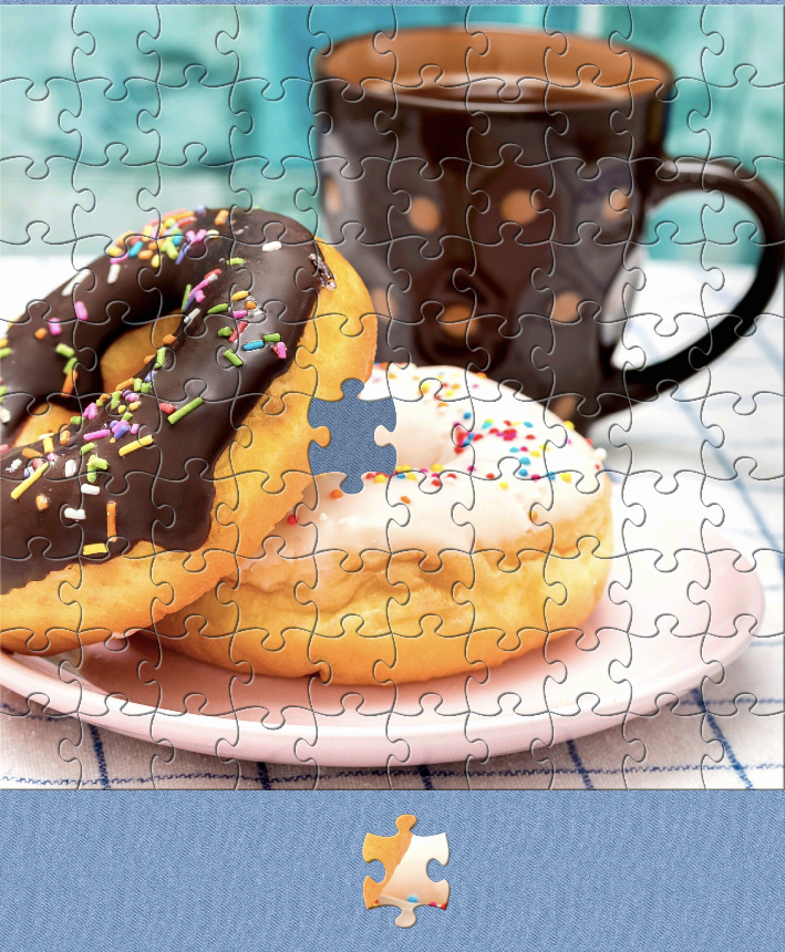
Luckily, technology has caught up, and now I happily spend my downtime playing jigsaw puzzles on my phone. One day, I noticed that when looking at only the edge pieces, I could see two pieces that were obviously a match next to each other.

I realized that this wasn’t the first time - I usually see two matching pieces next to each other. What are the odds? I marveled.

Obviously I needed to calculate that.

Step 1: Create a mathematical Question

My favourite difficulty level of jigsaw puzzle is a 15 by 15 puzzle which contains 225 pieces, of which 58 are edge pieces (feel free to count, it’s fun!). I started by asking a more mathematical question: If I reorder the numbers between 1 and $n$, what is the probability that my sequence contains at least one consecutive pair? (In my favourite case, $n$ = 58).

Step 2: Run a simulation to find experimental results.

Sometimes it’s a good idea to create a simulation and run several repetitions. You can use any method for this, and honestly, it’s easy to sometimes just use Excel to run some quick simulations. I’m writing this in R, so I might as well use that:

count_neighbours <- function(n){
  ## create a vector that has all the numbers from 1 to n, scrambled
  puzzle <- sample(c(1:n),size=n,replace = FALSE )

  ## are there neighbours?
  ## shift each number a bit
  puz_1 <- c(puzzle,n+100)
  puz_2 <- c(n+100, puzzle)
  difs <- abs(puz_1-puz_2)
  sum(difs ==1)
}


Repeat_experiment <- function(n,reps=1000){
  no_neighbours <- c(1:reps)*0
  for (i in 1:reps){
    no_neighbours[i] <- count_neighbours(n)

  }
  prop <- sum(no_neighbours>0)/1000
  m <- mean(no_neighbours)

  ##note: I put some extra returns in here in case I wanted more details later.

  return(list("vector"=no_neighbours, "proportion" = prop, "mean"=m))
}




##check with n = 58, and 1000 reps
Repeat_experiment(58)$proportion

## [1] 0.856

I ran this with different $n$ values, and discovered that once $n$ got big enough (say 10 or more), it seemed to always give and answer between 85% and 90%. Interesting. But it must depend on $n$, yes?

Just for fun, let’s try a few values of $n$:

Repeat_experiment(50)$proportion

## [1] 0.86

Repeat_experiment(100)$proportion

## [1] 0.872

Repeat_experiment(500)$proportion

## [1] 0.879

Repeat_experiment(1000)$proportion

## [1] 0.857

Repeat_experiment(10000)$proportion

## [1] 0.858

Step 3: Find a Probabilistic Answer

First, we need a bit of math. I’ve treated each puzzle piece as a number between 1 and $n$, assembling the pieces in a straight line. If I wanted to be 100% correct, I would have done the above work modulo $n$, that is, note that $n$ is next to 1. But that should not make a big difference. Mathematically, we have the following:

• There are $n!$ possible orderings of $n$ objects.
• There are $n$ consecutive pairs [note $n-1$ if 1 isn’t next to $n$ ]
• There are $n \choose 2$ (n choose 2) possible pairs of puzzle pieces.

Thus:

\(\text{Number of possible pairs}= {n \choose 2} = \frac{n!}{2(n-2)!}= \frac{n(n-1)}{2}\) If I choose two pieces at random, the odds of them being consecutive are:

Back to the puzzle:

We are working in a binomial distribution with the following parameters:

• $n-1$ as the number of trials (that is, the number of possible pairs in my sequence)
• $\pi= \frac{2}{n-1}$ is the probability of success; And
• I am looking for $P(X \geq 0) = 1- P(X =0)$:

So:

For n = 58, we have: \(P = 1- \left(1-\frac{2}{57}\right)^{57} = 0.8694411\)

1-(1-2/57)^57

## [1] 0.8694411

But what if $n$ is big?

Now we have:

1-exp(-2)

## [1] 0.8646647

Around 87%.

Step 4: Generalize a bit

As I proudly presented this to my family at dinner time, my kid wisely asked: “What about the whole puzzle? Not just the edges? Puzzle pieces touch four others - so would you multiply the answer by 4?”

Good question kid! No, but as it turns out - close! I guess eating all of those puzzle pieces really helped them be tuned into jigsaw puzzles.

Let’s start with an $n$ by $m$ puzzle. This puzzle has $n(m-1)+m(n-1)$ possible matches. Confused? Look at this nice image:

So we have the following numbers:

• $n$ columns and $m$ rows
• $m\times n = mn$ total pieces
• When we display the pieces in a row, there are (nm-1) possible pairs.
• There are $n(m-1)+m(n-1) = 2mn-n-m$ total pairings of pieces that fit together.
• There are ${mn \choose 2} = \frac{mn(mn-1)}{2}$ possible pairings.

That means that if I select two pieces at random, the probability that they are pairs (ie, they fit together) is:

So let’s fit that into a similar binomial distribution:

Thus: \(1- {(mn-1)\choose {0} }\times \frac{2(2mn-n-m)}{mn(mn-1)}^0 \left(1-\frac{2(2mn-n-m)}{mn(mn-1)}\right)^{mn-1}=1-\left(1-\frac{2(2mn-n-m)}{mn(mn-1)}\right)^{mn-1}\)

For my 15 by 15 puzzle, (ie, (m=n=15)), we have:

So: \(1- \left(1-\frac{2(2mn-n-m)}{mn(mn-1)}\right)^{mn-1} =\left(1-\frac{2(420)}{225(224)}\right)^{224} = 0.9768276\)

1-(1-(2*(2*225-30))/(225*224))^(224)

## [1] 0.9768276

But I like to generalize! Let’s say this is a really big puzzle. For simplicity’s sake, let’s make it an $n$ by $n$ square. As $n$ grows large, we have:

1-exp(-4)

## [1] 0.9816844

So in this case, I really would expect to see at least one match!

Conclusion

One conclusion is “Amy! You have too much time on your hands! Don’t you have enough actual work to do?” I do, but sometimes it can be fun and satisfying to take a small question, and expand it to a larger question. Did I learn something about jigsaw puzzles? Probably not, but I did have a lot of fun!

But look at what we did here! We asked a simple question, and then expressed it mathematically. We took that mathematical question, and used simulation to come up with a hypothesis. We then used some basic counting and probabilities to come up with a parametric answer - that is, an equation where we just had to sub in $n$.

I hope you enjoyed.